https://huggingface.co/spaces/nanotron/ultrascale-playbook
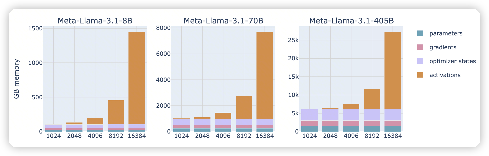
一上来有一个memory usage breakdown的图，展示了不同参数下，各个部分占用比重。

Memory usage breakdown

llama3 8B

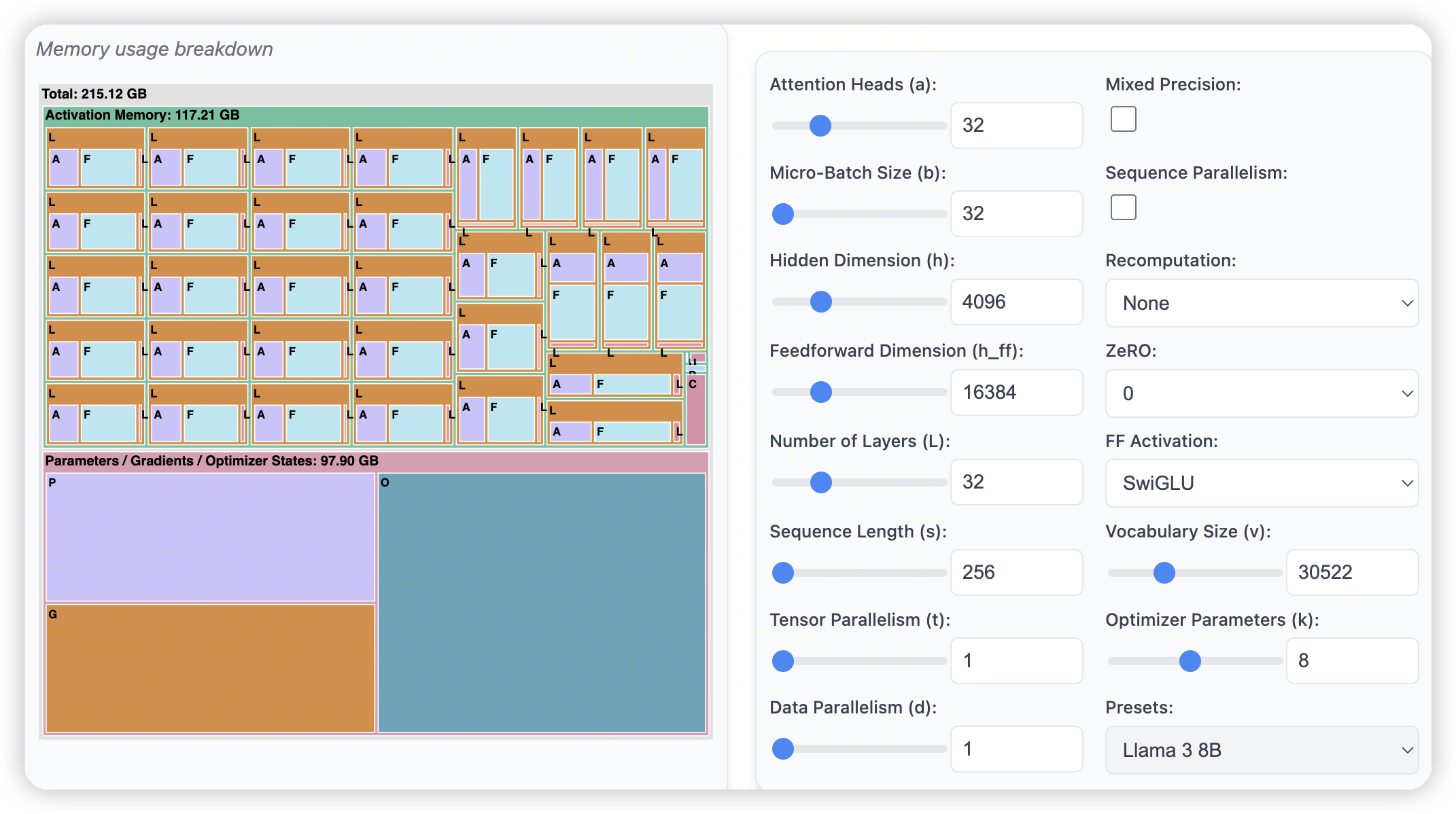
• 256的sequence length

• 打开mixed precision可以缩小activation memory。这里大概是认为从FP32变成了FP8，所以activation memory减少到了28G

• 打开zero后，P/G/O占用的内存会随着data parallelism degree逐步下降

• 不过这里好像有个bug，调整TP并没有节省P/G/O的内存占用。只对activation生效了。不过实际上应该是有帮助的

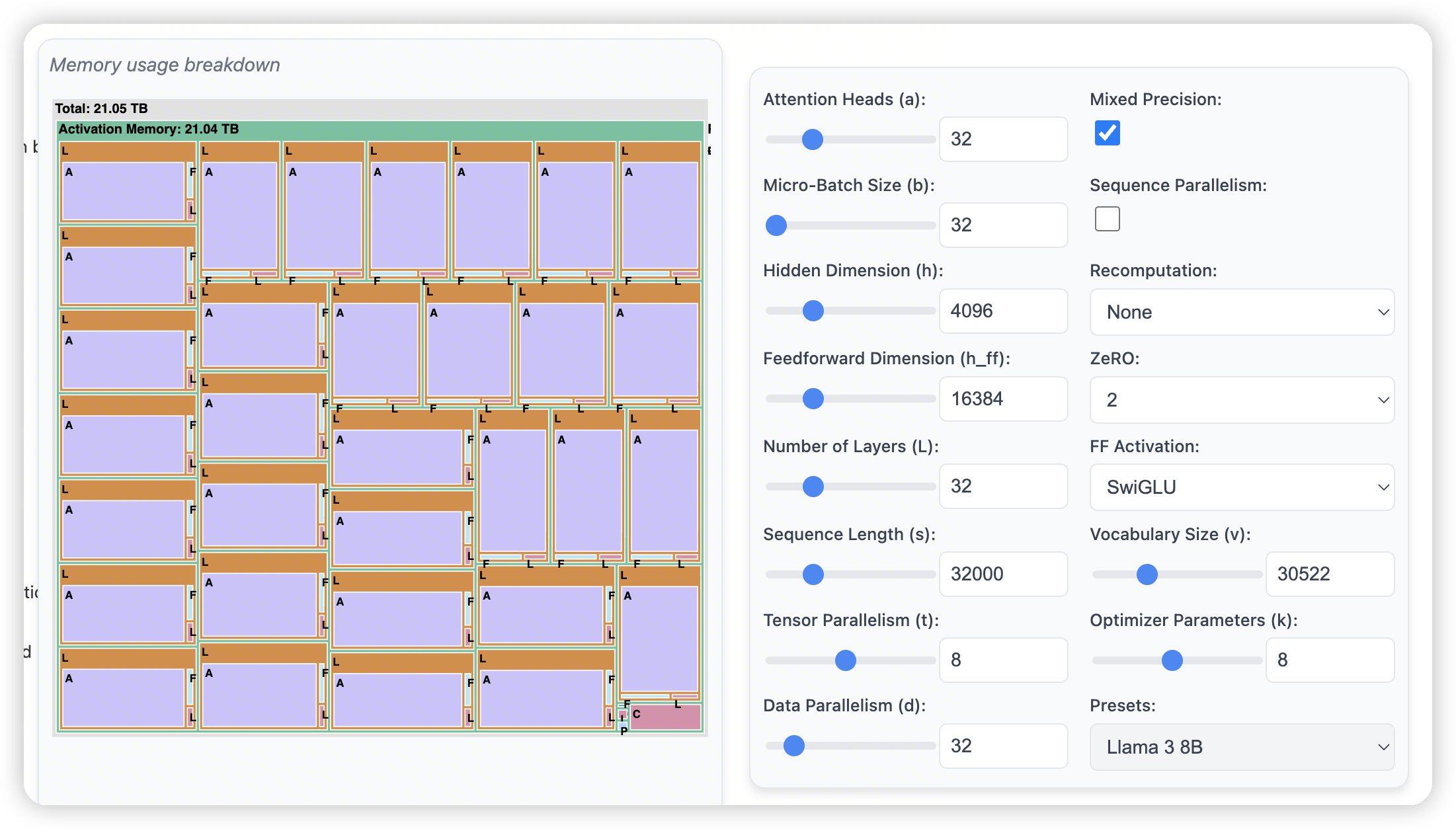
• 进一步调整sequence length。32k的时候，activation memory占了绝大多数的内存。

• 从这里可以看出来内存占比，绝大多数的内存都被attention吃掉了。

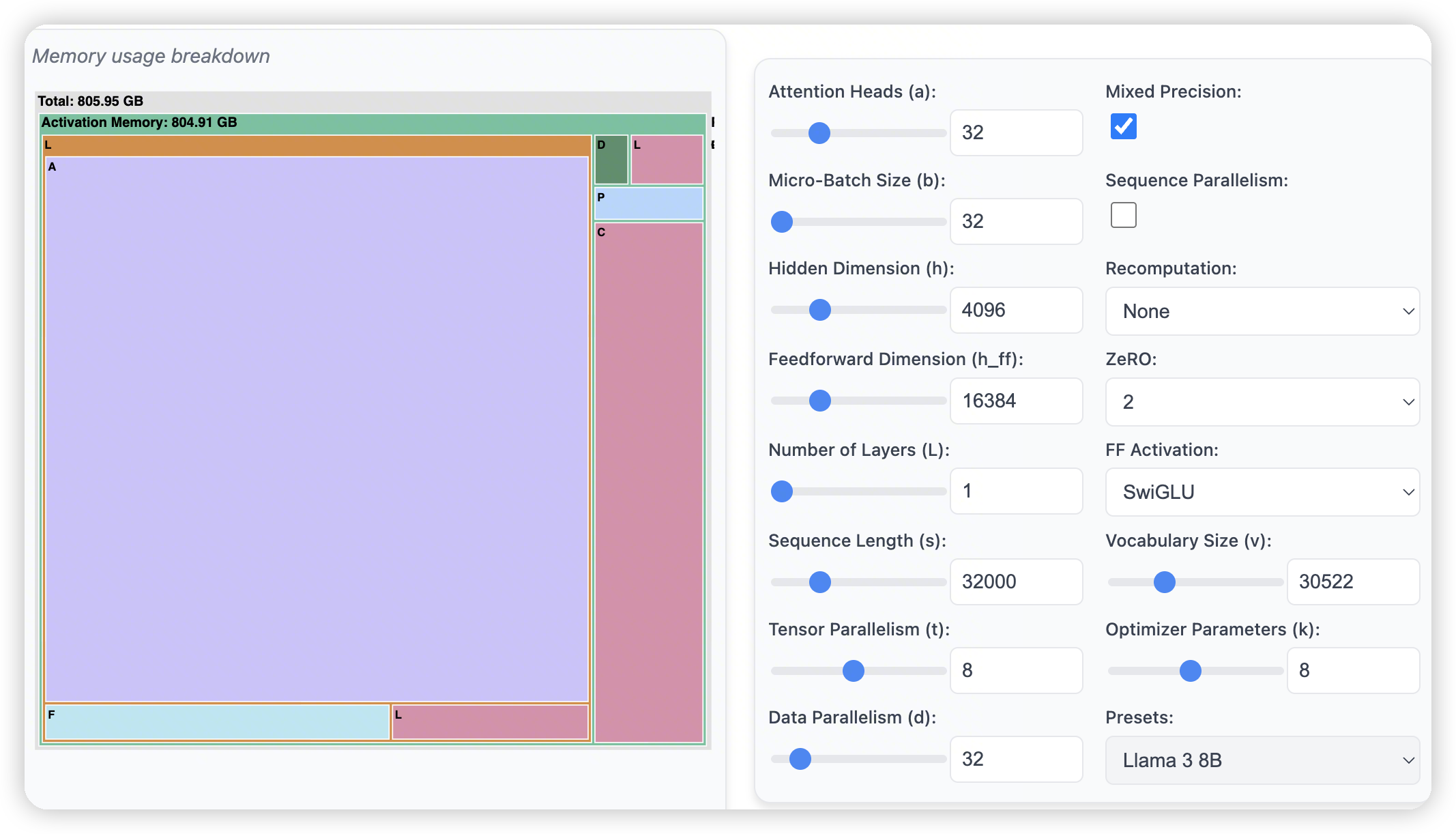
• 不过在32k的 context length下。layer norm，dropout这些也都吃了十几个G，也是不小的开销。

  • 所以每一步都需要优化

  • 启动SP之后，可以优化layer norm这些，让他能够随TP维度扩展

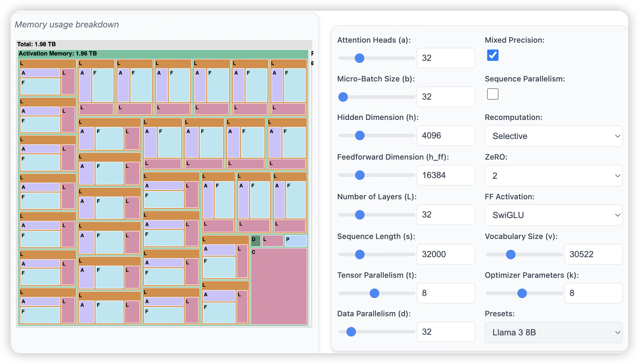
• 开启了recomputation后，可以再次缩减一下attention层的内存占用
  • 也可以看出来recomputation对attention层的贡献是更大的，因为attention层保存N方的score矩阵开销太大了。

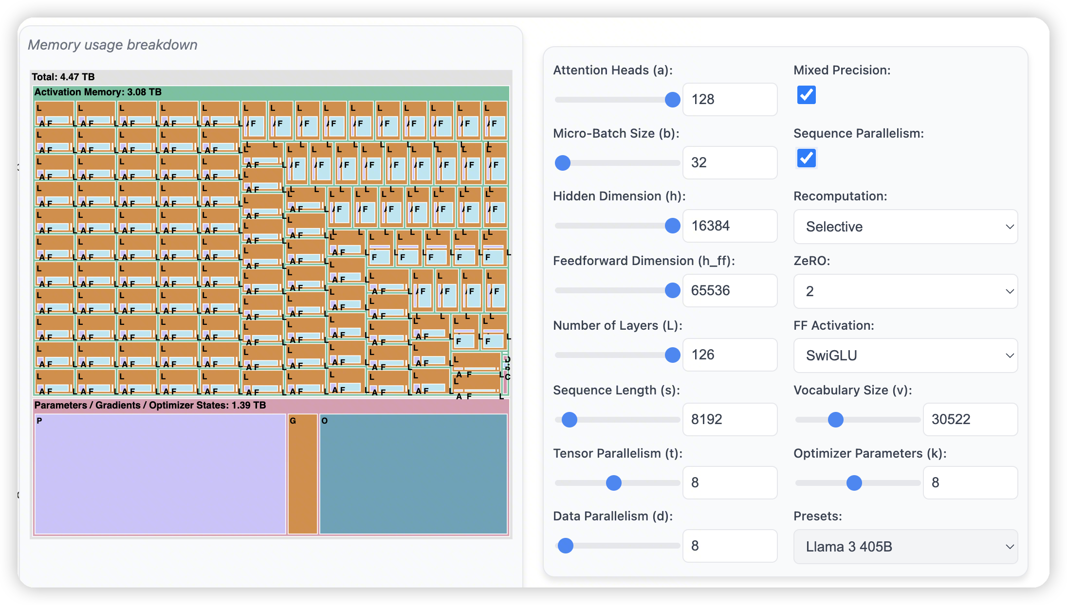
• 在一个常规的配置下，405B模型，8k的context length。开了sequence parallel + selective recomputation
  • 单个layer变成25G的activation。其中Feedforward占了17G，attention占5G

  • Context length变大也是类似的结果。内存占比的大头逐渐迁移到FFN中

• 此时如果再想拓展。可以通过CP来扩展FFN。或者是通过EP

这里还有一个更细粒度的：https://huggingface.co/spaces/nanotron/predict_memory

Cheatsheet

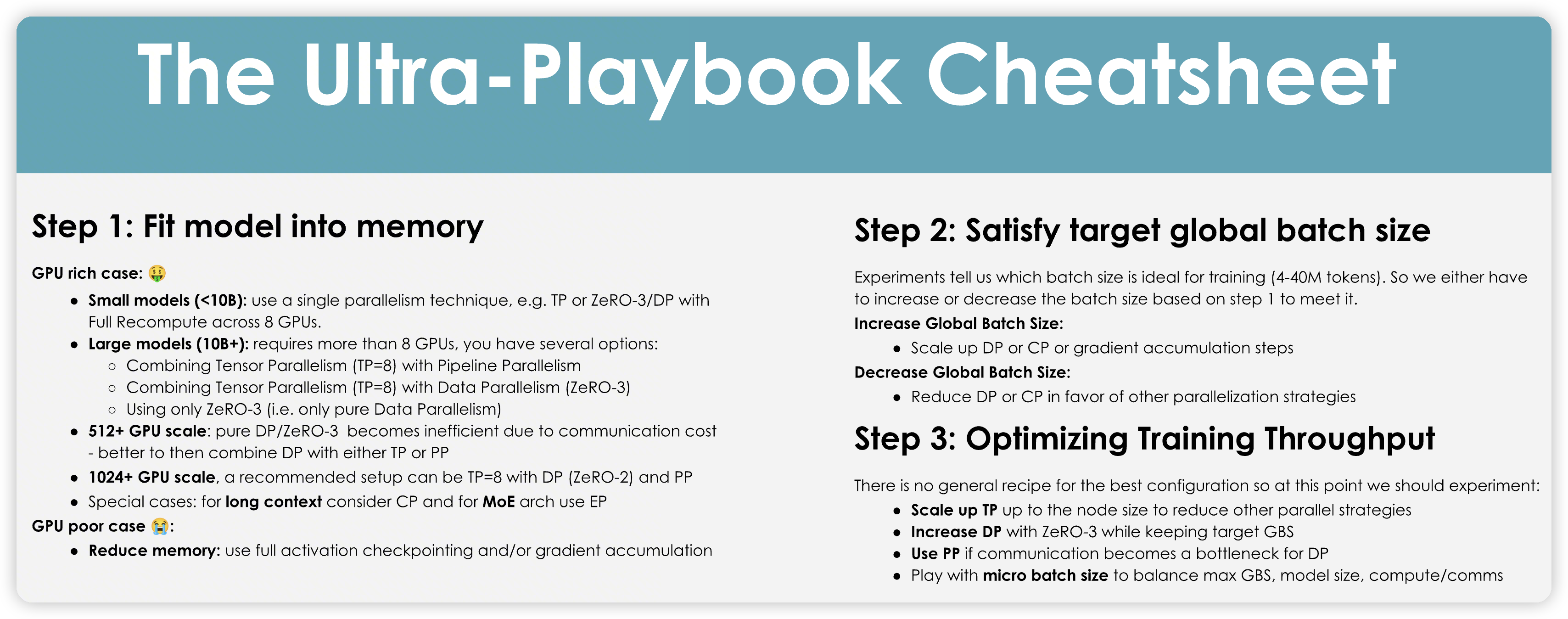
• 训练模型的第一步是把模型放到内存中
  • 小模型可以使用简单的并行策略

  • 大模型需要用TP + PP，以及ZeRO3来降低模型/activation的内存占用

  • GPU较多的场景，因为通信开销的原因，ZeRO3效率会降低

    

    • 当rank数量变多的时候，通信的瓶颈会从数据量转移到参与通信的rank数上。导致AG/RS开销不可忽略
  • 更大规模的GPU场景，推荐使用ZeRO2 + PP，对拓扑要求没那么敏感。
    • PP通信量低

    • 同时ZeRO2和PP没有ZeRO3的劣化问题

  • Long context，考虑使用CP

  • MoE架构，使用EP

• 为了提高样本效率，需要设置好合适的batch size。

  • 通过提高DP/CP的数量，来提高batch size
    • 或者是进行gradient accumulation。做多个microbatch

    • 这里感觉还需要考虑的是，如果切的microbatch太小了，会导致计算强度比较低，影响MFU

  • 降低DP/CP的数量，转移成其他的并行策略，来避免对batch size的依赖。

    • PP也会有影响。可能考虑做TP/EP
• 提高训练吞吐
  • 这块就是多种策略了，需要大量实验来跑

• 这里是bf16 + fp32的混合训练

• 对于模型来说，需要保存optimizer state，fp32的master weight，bf16的model weight，fp32的grad

• Compute = 6ND，对应这里的6 * model weight * token_num

  • 简单想就是每个token对模型做matmul，每个token对每个参数一次乘，一次加，就是2ND。

  • backward的时候一般认为是2倍的forward计算，涉及到grad_w/grad_x，所以总共是6ND

• DP
  • 需要吃batch size

  • 最简单的DDP通过减少单个GPU的batch size，来减少activation

  • 然后是ZeRO123，逐步减少model state相关的。同时引入更多的通信

  • 好处是一般可以进行overlap

• TP

  • 不吃batch size

  • activation/model state都能减少

  • 涉及到关键路径的AG/RS，因为当前layer的matmul计算得到结果后，才能做通信，并进行下一层的计算。

  • 这里说的overlap不确定是什么含义，感觉除了backward那里，forward好像overlap不了多少

• PP

  • 需要batch size来切microbatch，减少bubble

  • 切分模型，所以可以优化model state。虽然没有优化peak activation，但是总的activation（用于做backward的）还是减少了

  • microbatch虽然不影响总的通信量（非ZeRO3），但是会有算子启动的开销。

• CP

  • Model state是复制的，一般是和DP结合到一起。所以也可以应用zero那些策略。

  • 切分sequence，所以也减少了activation

  • 对于ulysses来说，引入了一个关键路径上的all2all，有额外的通信开销。同时需要吃head数量，因为是从sequence切分转化成了head切分。head不够的话，并行度就不够了。

  • 对于ring attention来说，因为分chunk的原因，实践中跑起来效果并不好。计算强度也不高。在USP中也有提到，表现一般没有ulysses好。

    • Ring attention有计算/通信的overlap
• EP
  • 如果MegatronLM的parallel folding的话，可以独立扩展

  • 引入了all2all。以及动态sequence的问题，可能影响计算效率

  • Shared moe和all2all可以做overlap，以及deepseek的dual pipe也可以做overlap

  • 感觉上应该是能用则用，因为MLP是计算大头

Training on One GPU

The batch size (bsbs) is one of the important hyperparameters for model training; it affects both model convergence and throughput.
A small batch size can be useful early in training to quickly move through the training landscape to reach an optimal learning point. However, further along in the model training, small batch sizes will keep gradients noisy, and the model may not be able to converge to the most optimal final performance. At the other extreme, a large batch size, while giving very accurate gradient estimations, will tend to make less use of each training token, rendering convergence slower and potentially wasting compute resources. You can find a nice early discussion of this topic in OpenAI’s paper on large batch training
[1]
, or in section 4.2 of the MiniMax-01 technical report.

• 小batch size导致gradient noisy，不容易converge to the most optimal final performance

• 大batch size会有非常好的gradient estimation，导致单个token的利用率不高。影响样本效率

  • 直观理解就是单个token无法贡献更多的gradient estimation了
• deepseek会在前469B token中，从batch size 3072慢慢增长到15360

需要注意的有关样本效率这块，并不是单纯说的训练中的一个sample算是batch size = 1，实际上这里的样本是batch size * sequence个，因为每一个token都是独立计算的。

A sweet spot for recent LLM training is typically on the order of 4-60 million tokens per batch.
The batch size and the training corpus size have been steadily increasing over the years: Llama 1 was trained with a batch size of ~4M tokens for 1.4 trillion tokens, while DeepSeek was trained with a batch size of ~60M tokens for 14 trillion tokens.

https://nanotron-ultrascale-playbook.static.hf.space/index.html#kernels
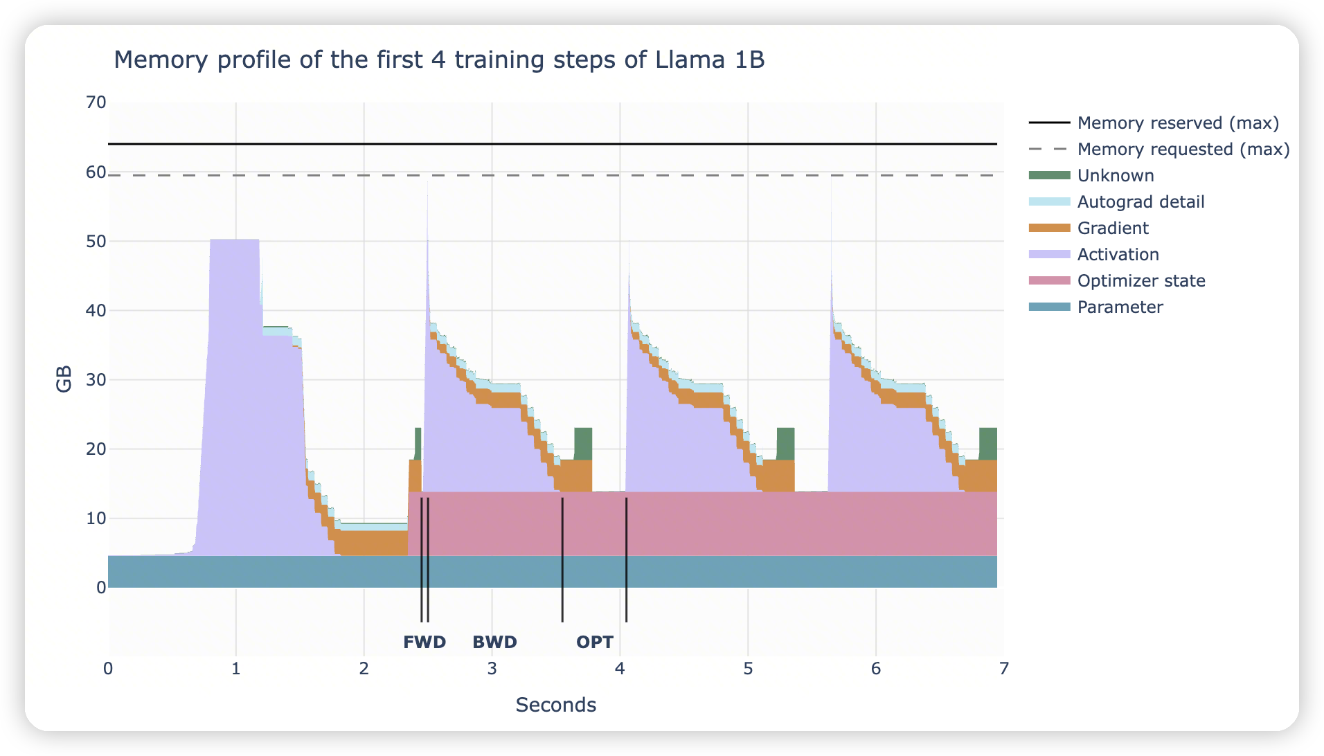
这里有记录profile相关的操作。
从图上可以看到：

• forward阶段非常的快，只有一个尖刺的内存占用

• backward阶段，逐渐释放activation，转化成gradient

• 常态化的param/optimizer state

Interestingly, mixed precision training itself doesn’t save memory; it just distributes the memory differently across the three components, and in fact adds another 4 bytes over full precision training if we accumulate gradients in FP32. It’s still advantageous, though, as computing the forward/backward passes in half precision (1) allows us to use optimized lower precision operations on the GPU, which are faster, and (2) reduces the activation memory requirements during the forward pass, which as we saw in the graph above is a large part of the memory usage.

• Mixed precision training，使用2byte的参数的时候，因为我们可能会用4byte的参数做grad accumulate，所以原本的grad/param变成2byte后，又加了新的4byte导致不变。

• 同时这里因为还会存全精度的param，所以还有4byte保留。这么看好像其实内存还增加了。

• 不过低精度的参数可以使用更快的计算操作，拥有更高的flops

• 同时减少了activation需要的内存，以及如果有通信的话，通信量也会减少。所以整体还是有收益的。

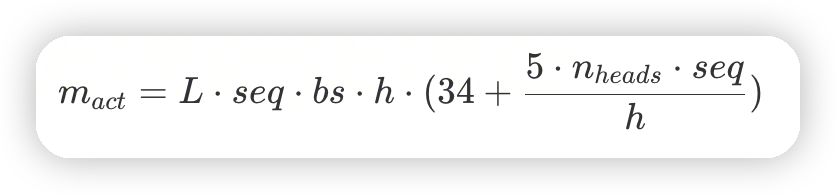
activation内存的计算，都是来自于megatron的第三篇论文，selective activation recomputation那个

for short sequences (or small batch sizes), memory usage for activations is almost negligible, but from around 2-4k tokens they start to take up a significant amount of memory, while usage for parameters, gradients, and optimizer states (as we’ll discuss later) is roughly independent of the sequence length and batch size.
For large numbers of input tokens (i.e., large batch sizes/sequences), activations become by far the largest memory burden.

这里也回顾了一下selective AC的策略：

• 对于attention层来说，占用了大量的内存，同时compute开销不大。

For a GPT-3 (175B) model, this means a 70% activation memory reduction at a 2.7% compute cost.

有关AC对于MFU的影响：

When you're measuring how efficient your training setup is at using your GPU/TPU/accelerator, you usually want to take recomputation into account to compute total FLOPs (floating-point operations) and compare this to the theoretical maximum FLOPS (floating-point operations per second) of the GPU/TPU/accelerator. Taking recomputation into account when calculating FLOPs for a training step gives a value called "hardware FLOPs," which is the real number of operations performed on the accelerator.
However, what really matters at the end of the day is the total time needed to train a model on a given dataset. So, for example, when comparing various GPUs/TPUs/accelerators, if one of these provides enough memory to skip recomputation and thus performs fewer total operations (lower hardware FLOPs) but still trains faster, it should be rewarded, not punished. Thus, an alternative is to compute what is called model FLOPS utilization (******MFU******), which, in contrast to HFU, only takes into account the required operations for the forward and backward passes through the model and does not include recomputation in the measured FLOPs. This value is thus more specific to the model than the training implementation.

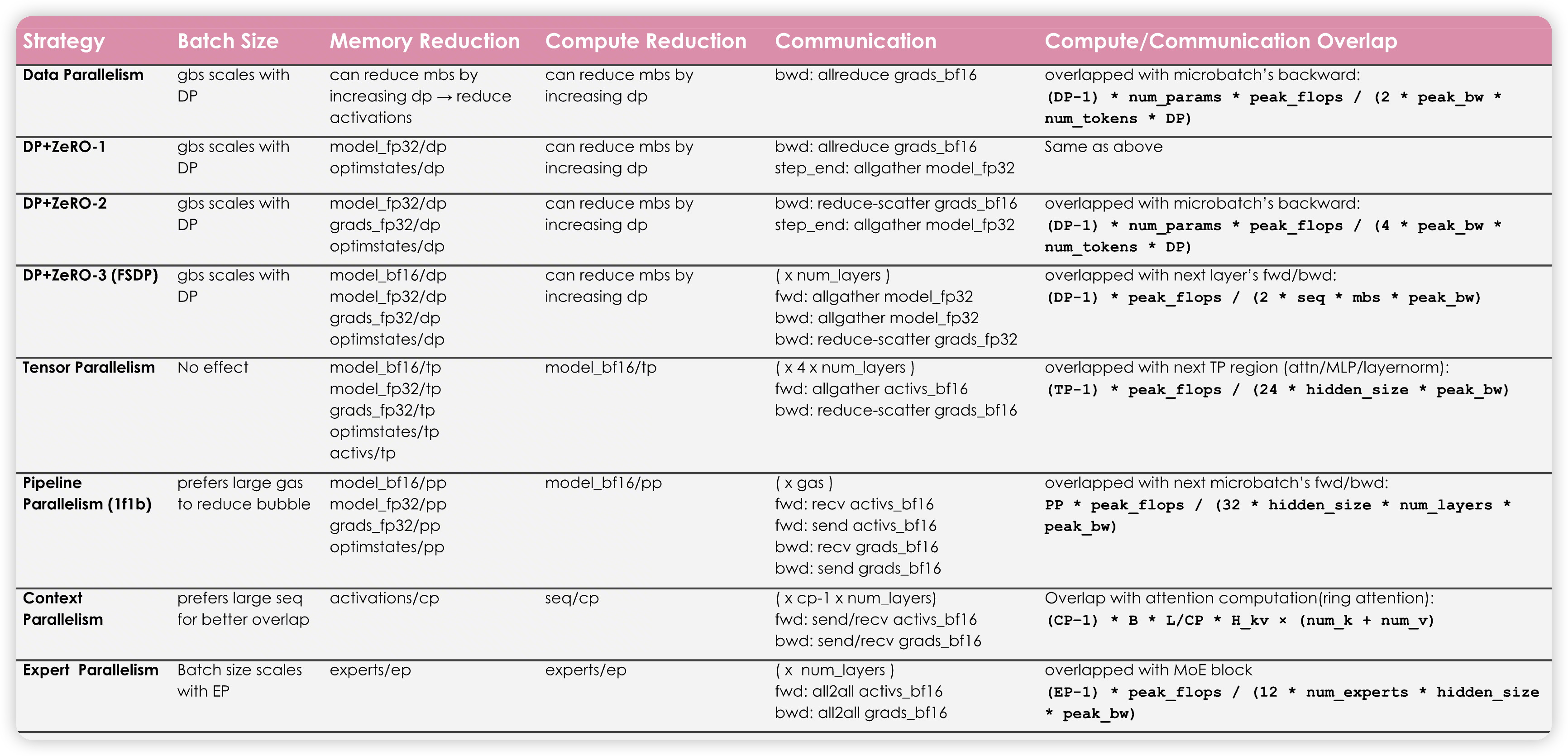
Data Parallelism

as we'll see, is just a parallel version of gradient accumulation.

最简单的DDP优化方法：

• Backward pass和all-reduce的overlap

• bucketing，减少通信开销

• 和gradient accumulation的配合，no_sync的时候不要触发all-reduce

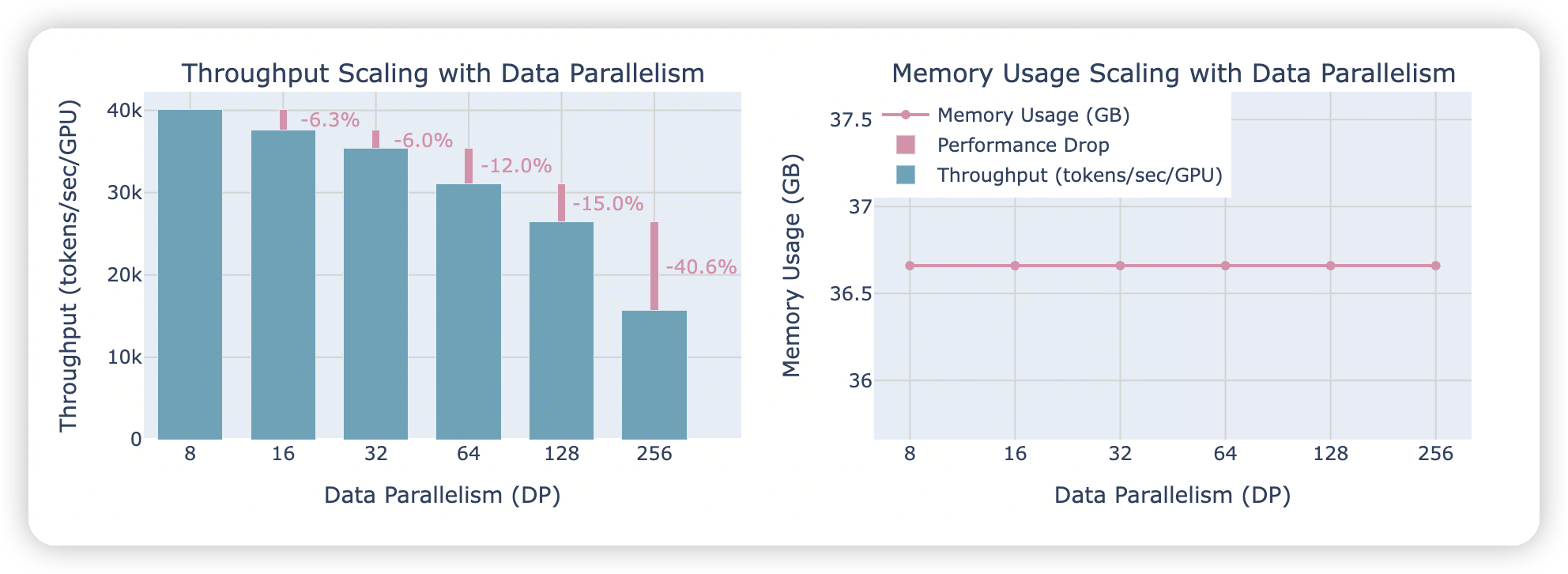
rank数量对DP的影响

后面这块主要讲的ZeRO，没有什么额外的，就不重复提了

Tensor Parallelism

就是Megatron那些，ColumnLinear和RowLinear
有一个额外的：

One interesting note about layer normalization in tensor-parallel training is that since each TP rank sees the same activations after the all-gather, the LayerNorm weights don't actually require an all-reduce to sync their gradients after the backward pass. They naturally stay in sync across ranks. However, for dropout operations, we must make sure to sync the random seed across TP ranks to maintain deterministic behavior.

TP这种有相同的输入，当操作相同的时候，需要固定部分操作的行为。

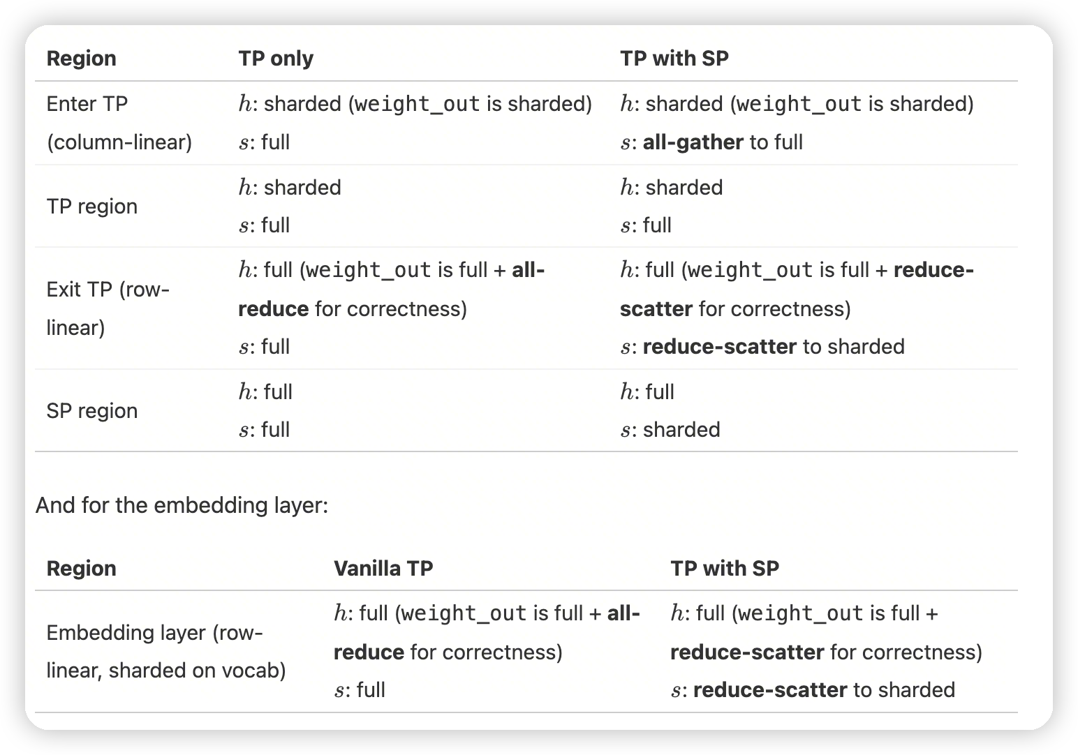
有一个偏实现方面的总结

Since LayerNorm layers in the SP region operate on different portions of the sequence, their gradients will differ across TP ranks. To ensure the weights stay synchronized, we need to all-reduce their gradients during the backward pass, similar to how DP ensures weights stay in sync. This is, however, a small communication overhead since LayerNorm has relatively few parameters.

这里提到了，layernorm这种point wise的，因为每个rank上输入的数据是不同的，所以梯度也不同。
最后需要做一下参数的all-reduce

顺便看了一下MegatronLM在这里的处理：

• _allreduce_non_tensor_model_parallel_grads中会对启动sequence parallel后，需要做梯度聚合的参数做处理。

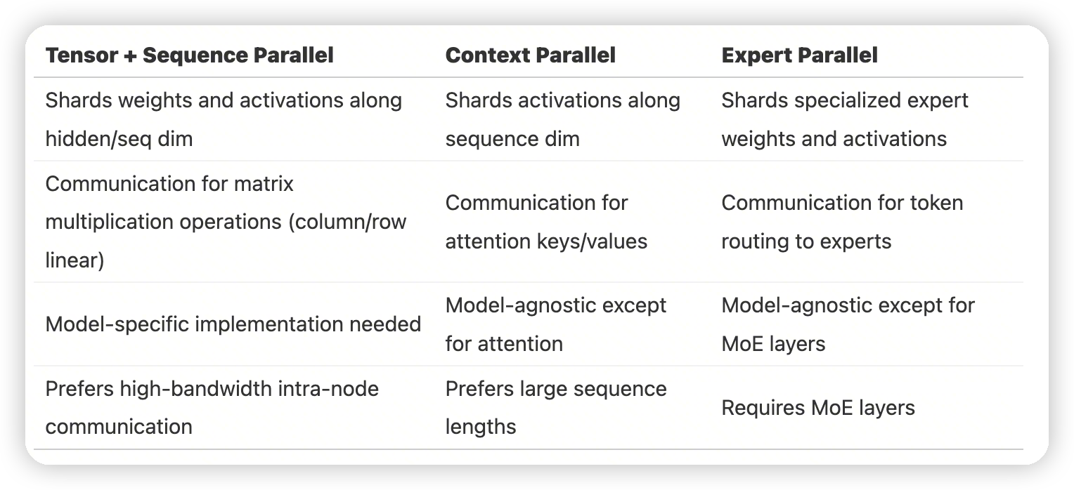
Context Parallelism

这一节主要讲的RingAttention + ZigZag做的负载均衡，没有额外的输入

Pipeline Parallelism

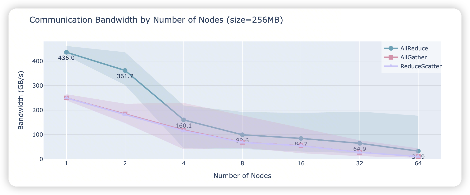
• 这里是benchmark了AR/AG/RS在多个node上的通信带宽。

• 可以看到在node变多之后，带宽下降还是比较明显的

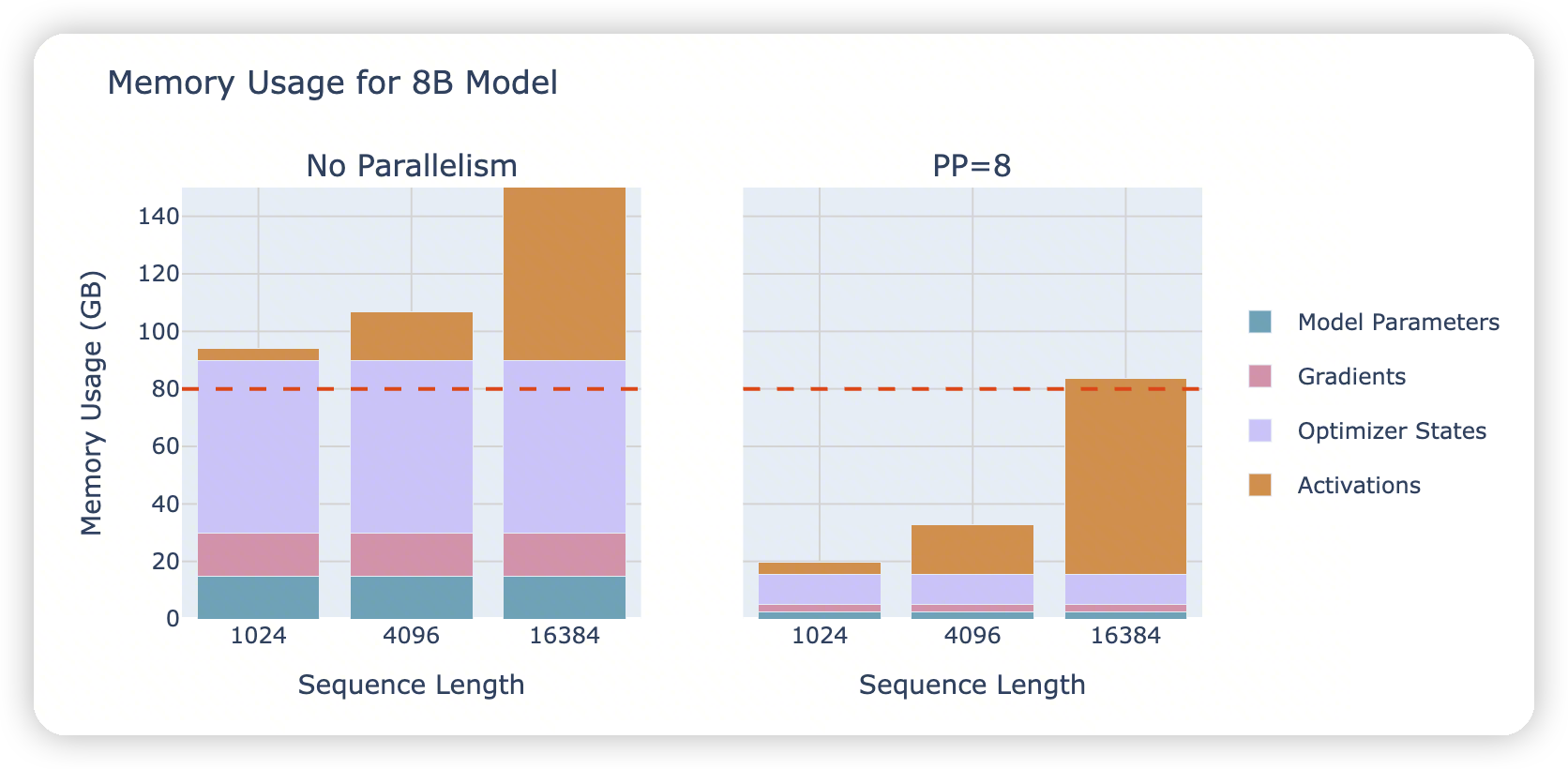
Looking at the figure above, we notice something interesting: while the model parameters are nicely split across GPUs, the activation memory remains the same on each GPU! which means we don't save any activation memory with this approach.

• 虽然PP切分了layer，但是这里没有节省activation的大小。

• 这里假设了是AFAB这种算法，相当于先把整个batch都forward了，再去整体做backward。

This is because each GPU needs to perform PP forward passes before starting the first backward pass. Since each GPU handles 1/PP of the layers but needs to process PP micro-batches before the first backward, it ends up storing PP×(activs/PP)≈activs, which means the activation memory requirement remains roughly the same as without pipeline parallelism.

• 这里说microbatch变多了，所以整体的activation没变化。但是感觉每个microbatch的activation应该变小了？

• 所以这里认为activation和batch size是无关的？需要再想想

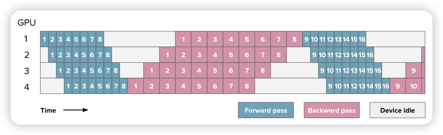
• AFAB，缺点是需要保存所有数据的activation

The general idea is to start performing the backward pass as soon as possible.

If you count carefully, you'll see that the bubble still has the same size, so our training efficiency is not significantly improved. However, we only need to store activations for p micro-batches (where p is the degree of pipeline parallelism) instead of m (where mm is the number of micro-batches), which can reduce the activation memory explosion we had in the AFAB schedule

1F1B并不会影响bubble size，而是减少了内存占用：

• 从m（micro batch的大小）减少到了p（pipeline parallelism degree）

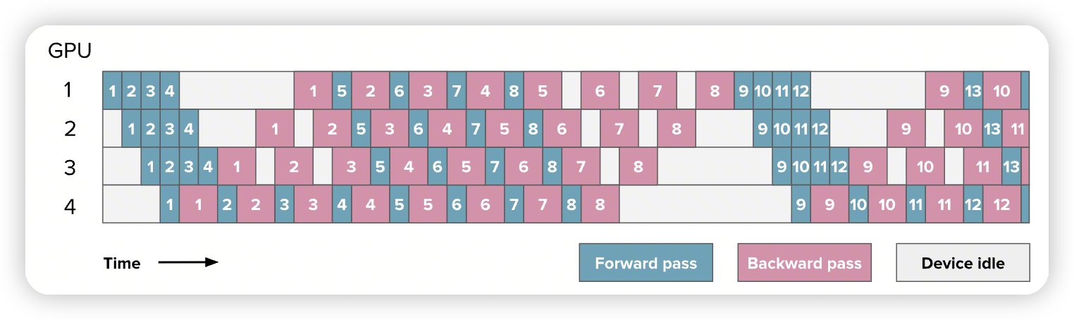
• Interleaved 1F1B，减少bubble size。从p - 1 / m减少到 p - 1 / m * v

• 通信量上涨了 v倍

• Activation memory上涨了一些，看rank0，额外forward了5, 6, 7这三个chunk

在megatron的代码中也可以看到，这里也提了。在interleaved 1F1B的时候，调度是有选择的：

• 比如rank0，可以选择执行新的一批microbatch。或者是选择执行之前的microbatch。

• 通过microbatch group size来控制

• Breadth-Fist Pipeline Parallelism paper中有详细建模这个事情

最后讲了一下zero bubble，和dsv3的拓展。

Expert Parallelism

这里没有讲太多EP相关的东西，对应的nanotron代码中也还没实现EP的

5D Parallelism

Both pipeline parallelism and ZeRO-3 are ways to partition the model weights over several GPUs and perform communication/computation along the model depth axis (for example, in ZeRO-3, we prefetch the next layer while computing). This means in both cases full layer operations are computed on each device, as opposed to with TP or EP, for instance, in which computations are performed on sub-layer units.

提了一下PP和zero3的冲突。很多其他地方也都提过这个

然后TP的缺点

• 带宽要求高

• 不是model agnostic

Best Training Configuration

这里和上面cheatsheet的一样

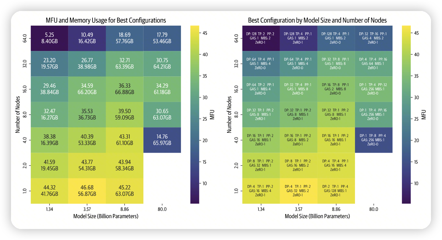
All the following benchmarks were conducted with a sequence length of 4,096 and a global batch size of 1M tokens. We gathered all the top configurations for each model and cluster size and plotted them in the following heatmaps

From this high-level visualization, we can draw several important insights:

• First, as we increase the number of nodes (higher parallelism), we observe a decrease in efficiency. This effect is particularly pronounced for smaller models, which have a lower compute to model size ratio. While we might typically compensate for small model size by increasing the batch size, we're constrained by our global batch size limit of 1M.
• Second, larger models present a different challenge. As model size increases, memory requirements grow substantially. This creates two scenarios with fewer nodes: either the model doesn't fit at all, or it fits but runs inefficiently due to operating near the GPU memory limits (see for instance the 80B parameter model training on 4 nodes).
• Finally, our benchmarks show how performance heavily depends on implementation quality. When we first implemented both parallelism strategies, tensor parallelism outperformed pipeline parallelism. After optimizing our PP code, it became the faster option. Now that we're improving the communication overlap in our TP implementation, we expect it to regain the performance lead.

做了一下benchmark，在不同的Node规模和model size上

• 小模型的MFU，随着parallelism的上升，降低的比较多。
  • 直观感觉就是PP/TP依赖模型的参数，小模型可能无法很好的scale

  • 如果依赖DP的话，还受限制于global batch size

• 大模型的瓶颈则在memory上。

  • 比如80B的模型在4 node上，训练效果比较差
• 最后还提了这些和实现关联性比较高
  • 所以更多的不是去考虑选择各种parallelism的方法，而是去做profile，然后去优化性能。

  • 不过选择parallelism的组合应该是大方向，然后再去优化内部的细节

从图上也可以看出来，并不是某种策略就是银弹了，需要在各种配置上做profile。需要做多种组合

• 不过发现好像没怎么用ZeRO2？

Lesson learned on benchmarking

So, the plan was simple: let's run every possible distributed configuration for every model and a number of cluster sizes. Even after excluding impossible configurations, we still needed to run thousands of experiments.
On paper, this sounds easy enough: we can easily launch big arrays of jobs on our cluster. However, as soon as we launched the first batches of experiments, our troubles began:

• PyTorch processes would sometimes fail to clean up properly.
• The Slurm job manager would forcefully terminate jobs, leading to node failures.
• Simple benchmarks that should have taken minutes would stretch into hours.
• Some jobs would hang indefinitely.

Running all the experiments in a finite amount of time required additional engineering, and we ended up spending a significant amount of time on things like:

• Minimizing cluster restart times and optimizing idle time
• Analyzing detailed NCCL debug logs
• Understanding memory usage patterns and CUDA memory allocator behaviors
• Improving pipeline parallelism performance on multi-node setups

These challenges taught us valuable lessons about the complexities of distributed training infrastructure. What looks simple in theory often requires careful attention to many moving parts in practice.

从这里可以看到，实际的distributed training还涉及到很多细节。这里提到的优化cluster restart time，分析nccl debug log，以及研究cuda memory allocator behavior/memory usage pattern都是比较宝贵的经验。

GPU

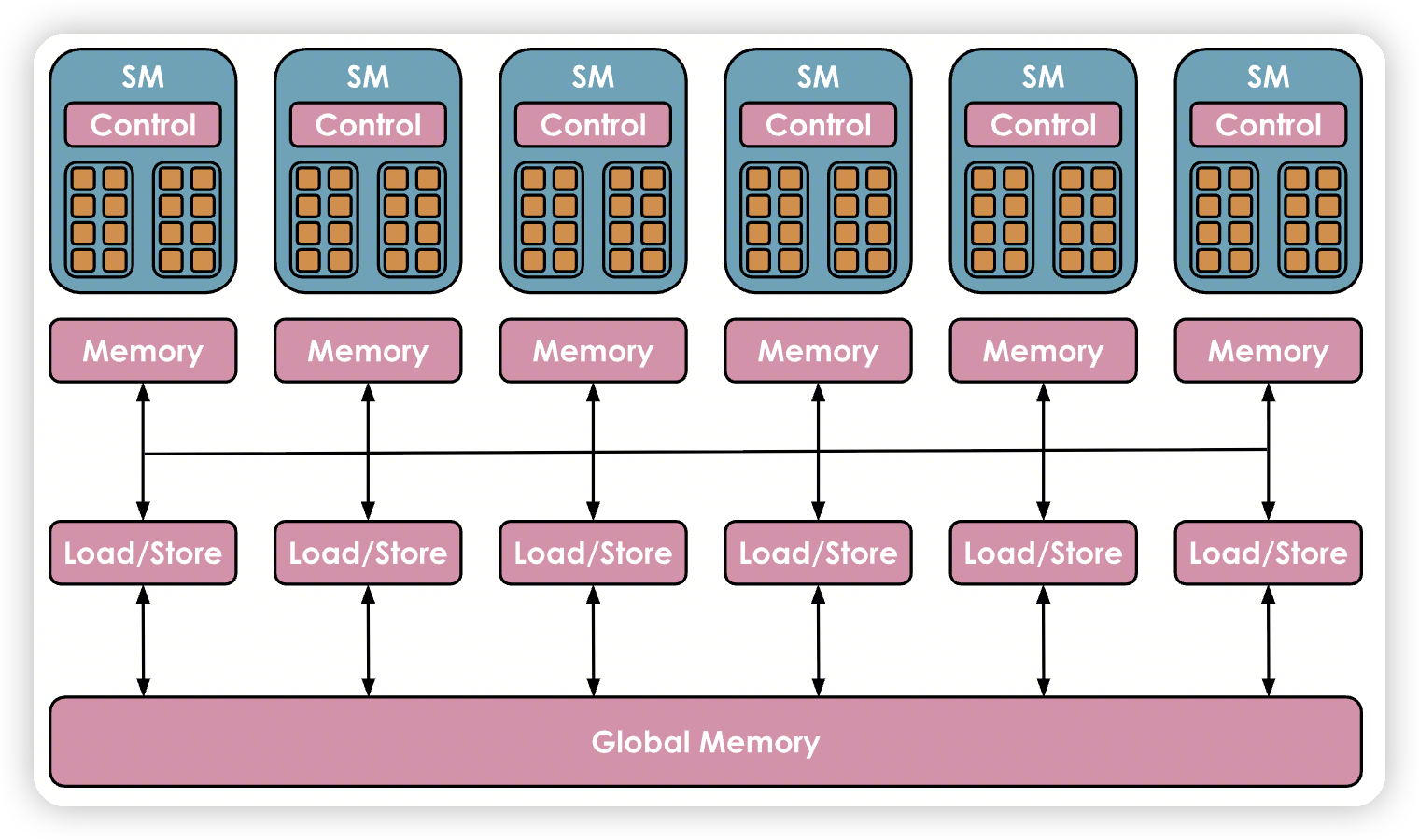
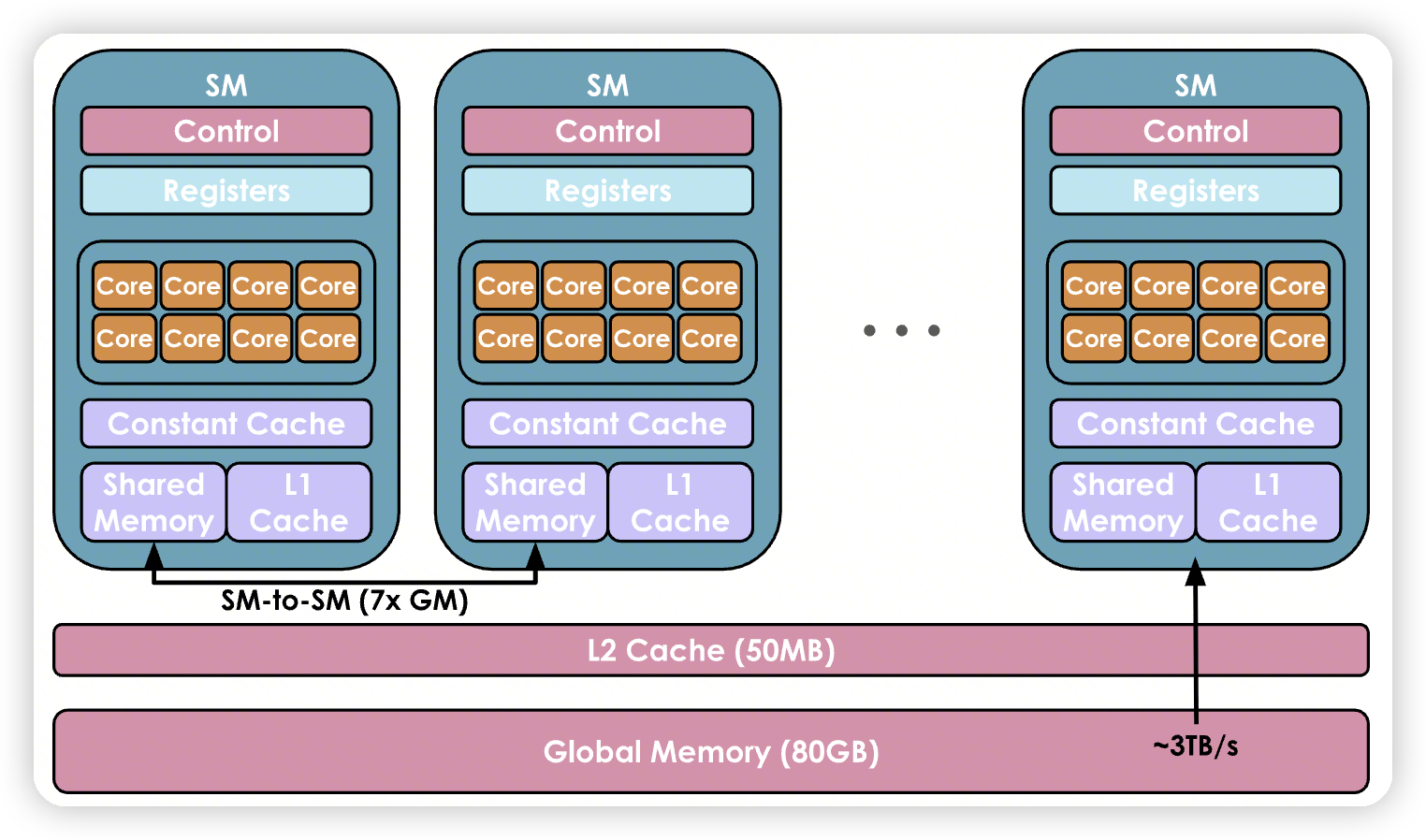
Registers are the smallest units and are private to the threads during executions. Shared memory and the L1 cache are shared between the threads running on a single SM. Higher up is the L2 cache shared by all SMs, and finally there is the global memory, which is the largest memory on the GPU (the advertised 80 GB for an H100, for instance) but also the slowest to access and query

SM级别的L1/SharedMemory
全局的L2 Cache/Global Memory

A piece of code running on a core of the GPU is called a kernel. It can be written at a high level in CUDA or Triton, for instance, and is then compiled to Parallel Thread Execution (PTX), the low-level assembly used by NVIDIA GPUs.

• GPU执行的代码叫kernel

• 高层语言可以通过CUDA/Triton来写

• 底层会被编译成交PTX的汇编，给GPU使用

• Threads are grouped in warps, each containing 32 threads. All the threads in a warp are synchronized to execute instructions simultaneously but on different parts of the data.

• Warps are grouped in larger blocks of more flexible size (for example, there may be 512 or 1,024 threads in a block), with each block assigned to a single SM. An SM may run several blocks in parallel. However, depending on the resources available, not all of the blocks may get assigned for execution immediately; some may be waitlisted until more resources become available.

• 32 thread组成warp，同步执行。会有diverge的问题

• 1024/512个thread组成block。一个block只能被一个SM执行。一个SM同时可以执行多个block。block是SM执行的单元

总结了几个优化的手段：

1. PyTorch: easy but slow

2. @torch.compile: easy, fast, but not flexible

3. Triton: harder, faster, but more flexible

4. CUDA: hardest, fastest, and most flexible (if you get it right)

Triton's capabilities are restricted to blocks and scheduling of blocks across SMs. To gain even deeper control, you will need to implement kernels directly in CUDA, where you will have access to all the underlying low-level details

• 这里提到了因为triton只能操作block，所以并不能达到和CUDA相同的能力

几个kernel的优化技术：

• Memory coalescing
  • 就是多个thread的访存做一下聚合
• Tiling
  • 利用shared memory做分块的计算。保证块内访问的都是高速的shared memory
• Thread coarsening
  • 这里提到的case是每个线程都在访问shared memory。因为线程太多，导致MIO pipeline过载

  • Thread coarsening的目的是减少线程数量，让每个线程执行更多的工作

  • 对于访存来说；trying to use fewer but wider loads

• Minimizing control divergence

  • 防止warp divergence

还有fuse kernel，减少访存。
以及mixed precision training。低精度的数据计算更快，带宽更低